SEPP65 solar access analysis with Rhino.Inside Revit

Over the past six years at Parametric Monkey, we’ve generated numerous ways to run solar access analysis for SEPP65 compliance. We’ve experimented with various workflows to find the simplest and most accurate method available. This tutorial will present what we believe is the best method to date – using Rhino.Inside Revit to provide accurate and fast results directly in Revit.

Background

When governments started mandating solar access analyses, such as those prescribed by NSW ‘State Environmental Planning Policy 65 – Design Quality of Residential Flat Development’ (SEPP65), architects turned to the ‘views from sun‘ method. Setting up an axonometric view parallel to the sun vector made it possible to see which parts of the building were receiving sun. However, the limitation of this method is that it couldn’t tell you how many apartments were compliant. Architects had to jump between various views and guestimate if the areas received the minimum amount of sun. Moreover, the camera views were often aligned by sight and weren’t very accurate. 

Seeing these challenges, we turned to Grasshopper and Ladybug as a means to improve efficiency and accuracy. Our first version focused on the conceptual massing stage. The script ran in Grasshopper, which meant that the model needed to be created in Rhino or imported into Rhino.

Following on from this, we created a detailed solar access analysis to run on individual rooms – much more in line with the actual legislative requirements. Revit geometry was extracted, the solar access analysis run in Grasshopper, and the results pushed back into Revit. While this method enabled yes/no compliance to be visualised and scheduled in Revit, it couldn’t provide the ‘heatmap’ visualisation within Revit.

Why not use Autodesk Insight or Dynamo?

Next, we explored the various options available to users wanting to stay within the Autodesk ecosystem. However, Autodesk’s Insight lighting analysis didn’t comply with SEPP65 requirements. Moreover, the Autodesk Visualisation Framework (AVF) used to visualise the results were transient, meaning results aren’t stored in the model – a tactic by Autodesk presumably to increase cloud credit churn. And finally, running the analysis directly within Dynamo was far too slow for large models. 

Rhino.Inside Revit

With the release of Rhino.Inside Revit, a whole bunch of new possibilities have now emerged. While it is still necessary to have Rhino installed, we can now run Grasshopper directly in Revit and create native Revit elements. This change means that we can now combine the computational power of Grasshopper with the BIM capabilities of Revit.

We can now combine the computational power of Grasshopper with the BIM capabilities of Revit.

Ladybug Tools 

In addition to switching to Rhino.Inside Revit, we’ve also revised the main computational logic by upgrading Ladybug, the go-to solution for environmental analyses. Back in November 2020, the Ladybug team released ‘Ladybug Tools’. This plug-in superseded the previous version, which has since been renamed to ‘Ladybug Legacy‘. The two versions are fundamentally different and generally not compatible. However, the two can be installed alongside one another without issues if you still have old scripts using the legacy plug-in.

As well as being more straightforward and faster, Ladybug Tools differs from the Legacy version in many ways. After much back-and-forth debating the best method, the ‘LB Sun Path’ component now returns vectors for the entire analysis period, making the solar access workflow far simpler. The legacy component, on the other hand, took the liberty of removing the last vector. As such, an analysis period of 9am to 3pm with 15min intervals would return 2:45pm as the last vector. To overcome this issue, an extra time step (15mins) needed to be added to the analysis period. This, in turn, complicated the heatmap visualisation and compliance calculations. However, this is all now much easier in the latest version of Ladybug.

The Ladybug team also develops Pollination, which allows you to run your simulations in the cloud. Pollination is fully compatible with the Ladybug Tools plugins (v1.3.0 and above), allowing you to reuse all your existing Grasshopper scripts with minor modifications. However, this tutorial is based on the Ladybug Tools plugin. 

Workflow

Taken as a whole, the revised workflow is far more comprehensive. Heatmaps can now be visualised within Revit, grid convergence is now included for accurate sun vectors, and best of all, results can be exported to the City of Sydney supplied compliance spreadsheet. Due to the nature of working with Revit, the workflow is a little involved but far faster and accurate than other methods.

Step 1 – Installation

Ensure you have Rhino 7 and Rhino.Inside Revit v1 installed. Refer here for detailed instructions.

To install Ladybug Tools, you can use the free, single-click installer for Pollination. While you might not want to run cloud-based simulations, the installer bundles in the Ladybug Tools plugin as well as the simulations engines, such as Radiance (daylight and solar simulations) and OpenStudio (energy simulations).

Alternatively, you can download LadybugTools from the Food4Rhino website. The latest version is 1.6.0. Ensure you do not use version 1.1.0, as it includes bugs that will cause the script to fail. Next, follow the installation instructions here. This is a bit of an involved process and can take some time. 

Once installed, you should be able to see the ‘Ladybug’ tab in Grasshopper. However, when using Ladybug Tools with Rhino.Inside Revit, many users have reported Ladybug not being able to find the Ladybug Python libraries. To resolve this issue, simply run the Ladybug installer directly with Rhino.Inside Revit.

Next, we need to install TT Toolbox by CORE studio. This plug-in enables us to export data to a preformatted Excel spreadsheet. The other plug-in we need to install is EleFront by FRONT Inc. This plug-in enables us to filter geometry by type (brep, mesh, etc.). Once downloaded, right-click and unblock, then place them in the Components folder. To find this folder location, go File > Special Folders > Components Folder.

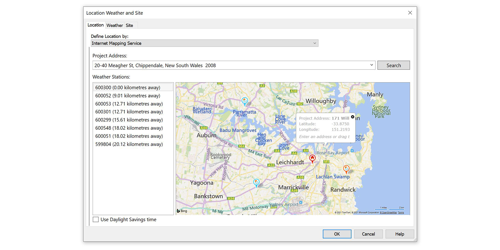
Step 2 – Set location

Before running the script, ensure that the Project Location has been set in Revit. Go Manage > Project Location > Location and set the project address. Note that the ‘use Daylight Savings time’ setting will not affect the script. 

Step 3 – Shared parameters

Ensure that the relevant project/shared parameters have been loaded into the project and assigned to the ‘Room’ category. By default, the script will search for:

• ‘Compliant Solar’ which is a yes/no parameter capturing if a room receives the minimum number of hours of sun to comply (typically 2 or 3 hours), and
•  ‘Zero Sun’ which is a yes/no parameter capturing if a room receives no sun whatsoever during the analysis period.

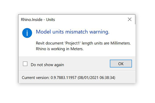
Step 4 – Set units to millimetres

Because the analysis is being conducted in Rhino and then pushed to Revit, we need to ensure the units are compatible. The latest versions of Rhino.Inside Revit now prompts you if this is not the case. Since our solar access script is set up for millimetres, we need to set both software to millimetres.

For Revit, go Manage > Settings > Project Units, and change the Length format to millimetres (mm).

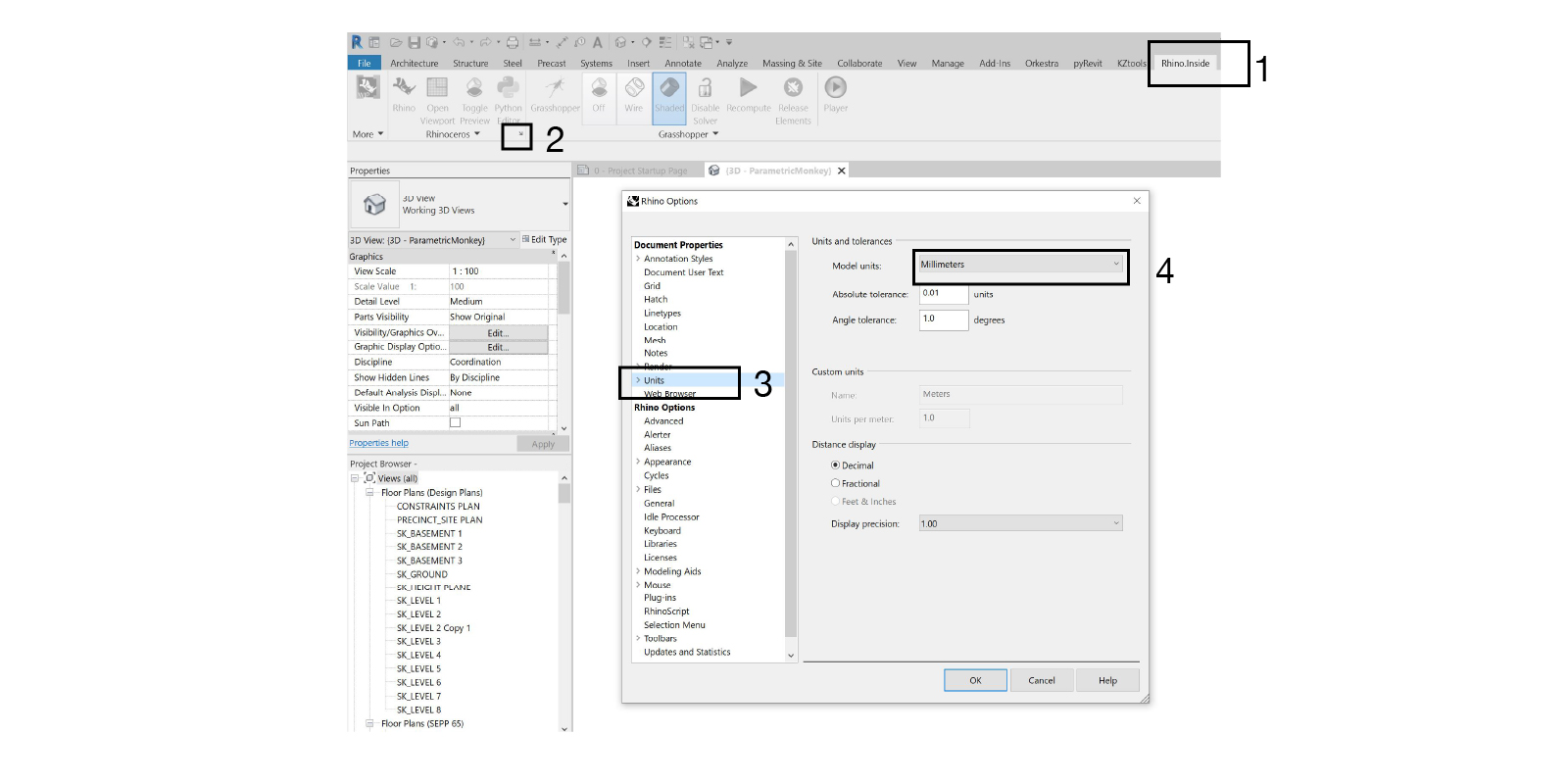
For Rhino, go Rhino.Inside > Rhinoceros > Rhino options (arrow in the corner) > Units, and set the model units to millimetres.

Step 5 – Prepare context

Within Revit, it is necessary to prepare the context for the solar access analysis. Context is defined as anything that will cast a shadow. The script enables two methods for referencing in linked geometry.

General requirements

The easiest way to prepare the context is to set up a 3D view from which elements are referenced. Using Visibility Graphics (VG) in conjunction with worksets and/or filters, turn off any unnecessary geometry. Essentially all we require are party walls, floors and roofs. Extraneous geometry such as planting, furniture, doors and mullions can all be hidden.

Glass balustrades, windows and glazing should also be excluded. However, since these are often modelled as walls, you will need to set up a filter to turn off only the glazed elements and not all the walls.

It is critical that the context model be as clean and minimal as possible to minimise computational time later in the workflow.

Option A: Specify individual links

This option allows the user to specify which elements to reference from within the current model. Up to four links are supported. However, if the linked models have been ‘split out’ from a single model, all the models will have the same document ID and cause this method to fail.

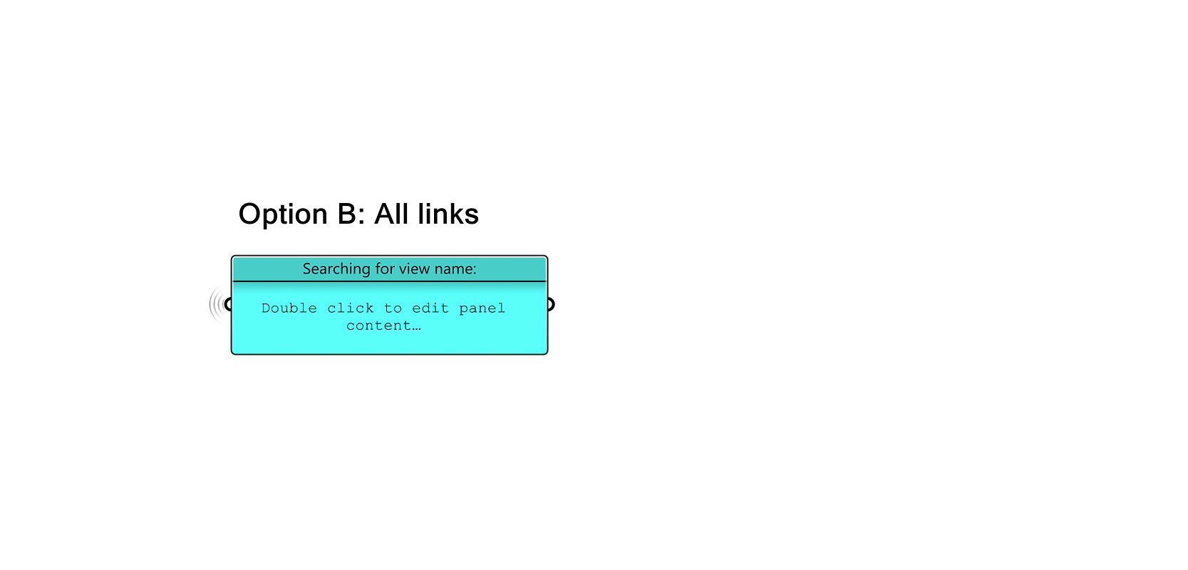
Option B: All links

This option will get all links automatically and search for a 3D view of the same name in the linked model. The geometry visible in that view is used as the context. Therefore ensure that the view exists in the linked models and that the visibility settings are correct.

Step 6 – Prepare analysis geometry

The script enables three methods for referencing in analysis geometry:

Option 1: Rooms

Ensure that all rooms to be analysed are bound and don’t contain any self-intersecting rooms. Otherwise, they will be excluded from the analysis. (Refer to our Dynamo Room Check graph to automate this process). Moreover, since we are using Yes/No shared parameters to record compliance, rooms to be analysed cannot be in a model group.

By default, the script references the ‘Room Category’ key schedule parameter. Only rooms where the value of this field contains ‘TERRACE’ or ‘BED’ will be included in the analysis. Therefore, this parameter needs to be populated.

If you plan on exporting the results to Excel, then the room ‘Number’ parameter also needs to be populated. The value should match with the corresponding terrace/apartment room so that the pairing can be calculated.

There are some optimisations that can be made to speed up the compute time:

Tip #1: Ensure that any context geometry is not grouped
It takes far longer to extract nested elements and their geometry.

Tip #2: Eliminate the use of room separation lines
If the room geometry creates adjacent coplanar surfaces, Ladybug merges these, meaning they need to be separated out downstream, which is extremely slow. The best way to avoid this is to ensure rooms don’t touch one another by separating them with a wall.

Option 2: Massing

The script can be run on the building massing to undertake a preliminary analysis. In this case, simple massing should be used. The script will remove any bottom or top surfaces and use the side surfaces only.

Option 3: Areas

Ensure that all rooms to be analysed are bound and don’t contain any self-intersecting rooms. Otherwise, they will be excluded from the analysis. (Refer to our Dynamo Room Check graph to automate this process). Moreover, since we are using Yes/No shared parameters to record compliance, areas to be analysed cannot be in a model group. Only areas where the name matches the inputs (‘TERRACE’ and ‘BED’ by default) will be included in the analysis. Therefore, this parameter needs to be populated.

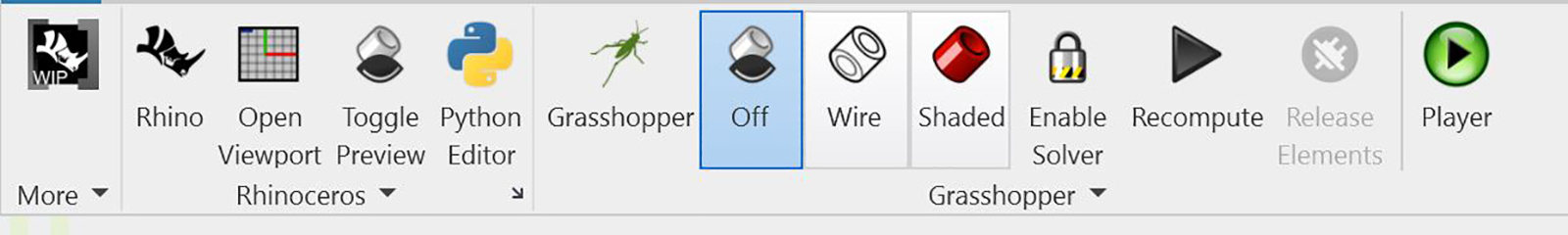
Step 7 – Disable Revit preview

Having the Grasshopper preview visible in Revit can dramatically slow down Rhino.Inside Revit. It is, therefore, recommended to set the preview to ‘off’ before launching the script. To do this, go Rhino Inside > Grasshopper > Off.

Step 8 – Define common settings

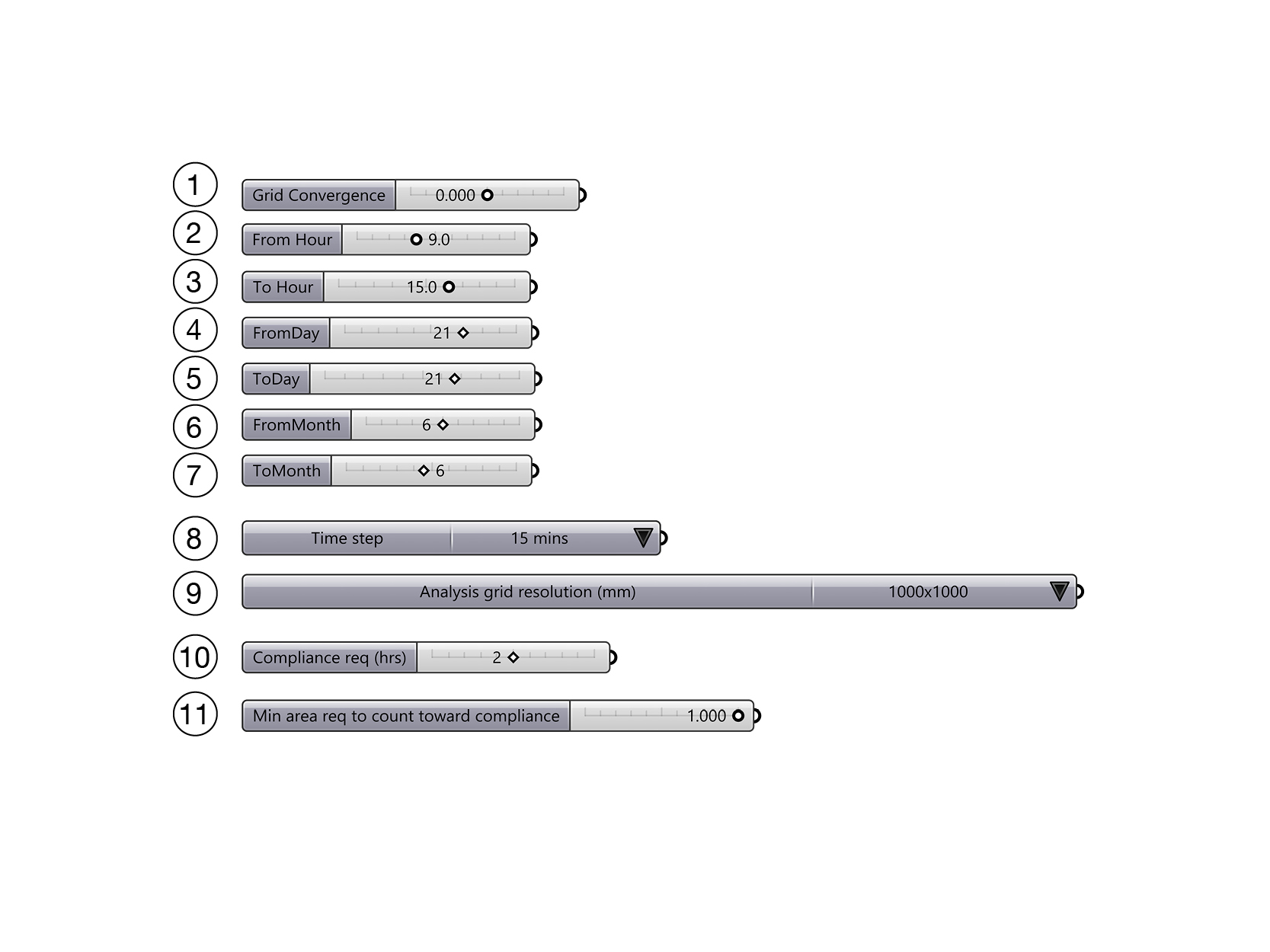
In Revit, open up Grasshopper and the solar access script. Remember that opening the file outside of Rhino.Inside Revit and saving it will cause the wires to break (as Rhino.Inside Revit components are only available within Revit). To run the script, first define the settings:

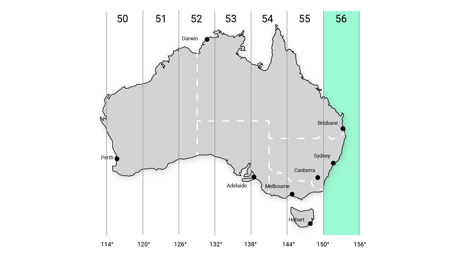
• Define the grid convergence (#1). If your model is orientated to True North, this value is 0. If your model is orientated to Grid North, such as GDA2020_MGA56, you’ll need to factor in grid convergence.
• Define the analysis period (#2-#8). By default, this is 9 am – 3 pm, 21 June.
• Define the analysis grid resolution (#9). Each analysis surface will be converted to a mesh with face dimensions approximately equal to this value. The lower the value, the higher the resolution of the analysis and the longer it will take to run.
• Define the number of hours required to comply (#10). The default is 2 hours.
• Define the minimum area required to count toward compliance (#11). The default is 1sqm.

True North

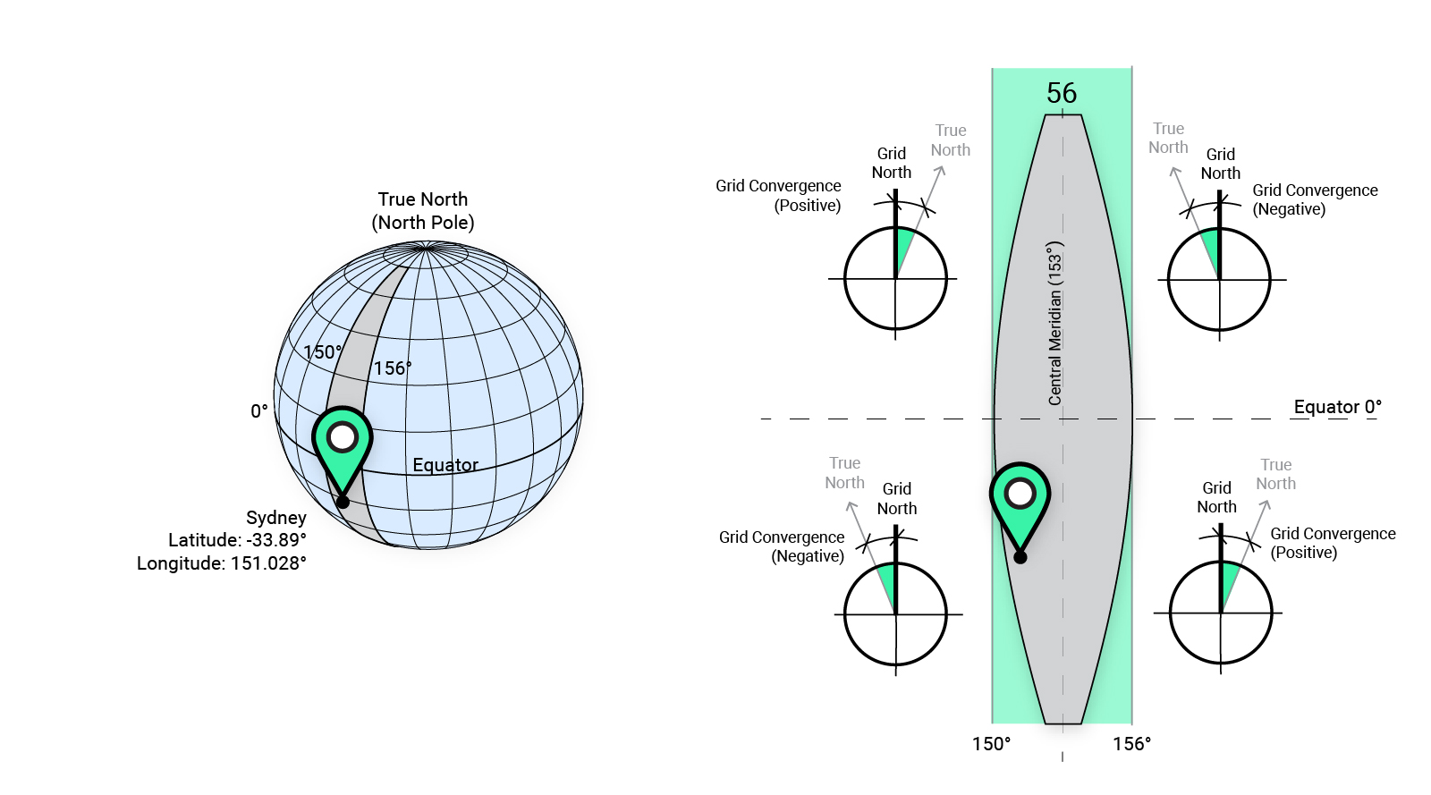
The script collects the Project Site Location and uses its latitude and longitude to create a Ladybug location. Next, the project’s Angle to True North is returned and combined with the grid convergence input to define north for Ladybug. If your Revit model is orientated to the real True North, that is, the direction along the earth’s surface towards the geographic North Pole, then the grid convergence is 0. However, if your Revit model is orientated to Grid North, such as GDA2020_MGA56, you’ll need to factor in grid convergence.

Grid convergence

Depending on the location, grid convergence and can be positive or negative. For the script, negative values indicate True North is to the West of Grid North, while positive values indicate True North to the East of Grid North. Sydney, for example, has a Latitude of -33.89° which means it is in the Southern Hemisphere and a Longitude of 151.028°, which means it is located to the West of the Central Meridian (153°) in MGA zone 56. This means that True North is West of Grid North, with an angle of approximately -1°. If your survey doesn’t contain this information, many government agencies publish Geodetic Calculators to assist in calculating the grid convergence.

Step 9 – Reference analysis elements

Common settings

• Define the analysis type (#12).
• Set the referencing 3D view (#13) to define the current phasing and if elements are visible in the view. For example, rooms that don’t match the view’s ‘New Construction’ phase will be filtered out. This view should have its detail level set to coarse to speed up the analysis process.

Option 1: Rooms

• Define the room name filters (non-case sensitive). Only rooms whose value contains this will be used in the analysis (#14 & #15). By default, the input includes ‘BED’ and ‘TERRACE’.
• Define the parameter name to reference (#16). By default, this is the ‘Room Category’ key schedule parameter.
• Define the offset from the floor (#17). This is the height the analysis mesh is offset. By default, this is 1000mm, as per the Apartment Design Guide.

Option 2: Building Massing

• Within your 3D context view, right-click on the select analysis geometry component (#18) and pick “set multiple graphical elements”, choose all of the massing elements, and then press “Finish”.

Option 3: Areas

• Define the area name filters (non-case sensitive). Only areas whose value contains this will be used in the analysis (#19 & #20). By default, the input includes ‘BED’ and ‘TERRACE’.
• Define the area scheme filter (#21).
• Define the offset from the floor (#22). This is the height the analysis mesh is offset. By default, this is 1000mm, as per the Apartment Design Guide. 

Compute

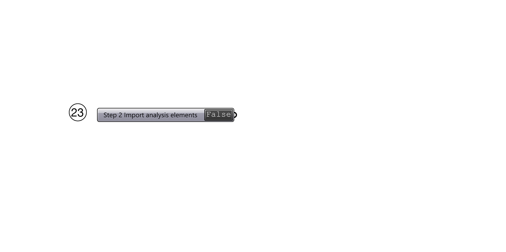
• Set the toggle (#23) to True to import the analysis geometry.

Step 10 – Reference project context

• Within your 3D context view, right-click on the “select building context” component (#24) and pick “set multiple graphical elements”, choose all of the project context (walls, floors, etc.), and then press “Finish”.
• Set the toggle (#25) to True to import the project context geometry.
• The script collects all of the element’s geometry and filters out anything which isn’t a brep or mesh. This means if you accidentally include model lines or levels, they won’t be included in the analysis. Note that the script will use the primary design option for each design set if design options have been used.

Step 11 – Reference linked context

The script enables two methods for referencing in linked geometry (#26). One only method can be used at any one time.

Option A: Specify individual links

• This option allows the user to specify which elements to reference from within the current model. Up to four links are supported. However, if the linked models have been ‘split out’ from a single model, all the models will have the same document ID and cause this method to fail.
• Within your 3D context view, right-click on the ‘select linked model instance’ component (#27) and pick “select one graphical element”, choose the linked model instances, and then press “Finish”.
• Within your 3D context view, right-click on the ‘select linked context elements’ component (#28) and pick “select multiple linked graphical elements”, choose all of the context elements (topography, massing, etc.), and then press “Finish”.
• Repeat the above steps for up to three more files (#29-#34), ensuring the data is in sync between the various instances.
• The script collects all of the element’s geometry and filters out anything which isn’t a brep or mesh. This means if you accidentally include model lines or levels, they won’t be included in the analysis.

Option B: All links

• This option will get all links automatically and search for a 3D view of the same name in the linked model based on input #13. The geometry visible in that view is used as the context. Therefore ensure that the view exists in the linked models and that the visibility settings are correct.

Compute

• Set the toggle (#35) to True to import the linked context geometry.

Step 12 – Run analysis

• Set the toggle (#36) to True to run the solar access analysis.
• Depending on the model’s size and the analysis grid resolution (#9), the analysis may take several minutes to run.

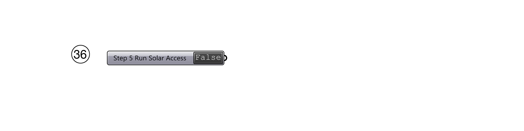
• Before proceeding to the next step, check the error panel to make sure everything is OK. There should be no errors shown.

Step 13 – Visualise results 

The script provides serval ways to visualise the analysis results.

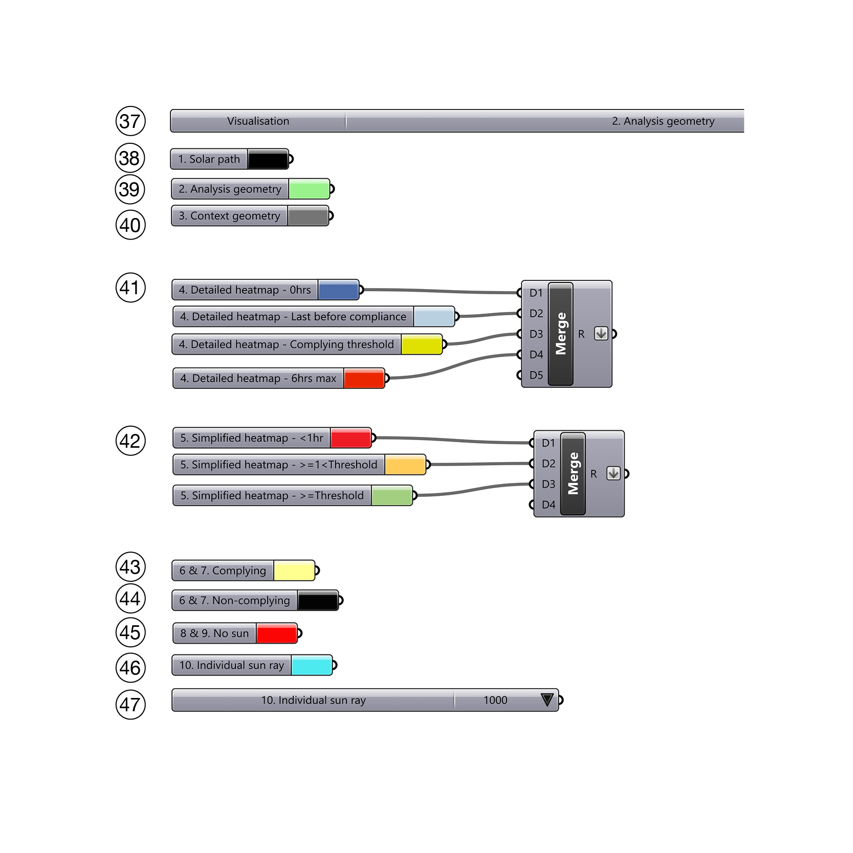
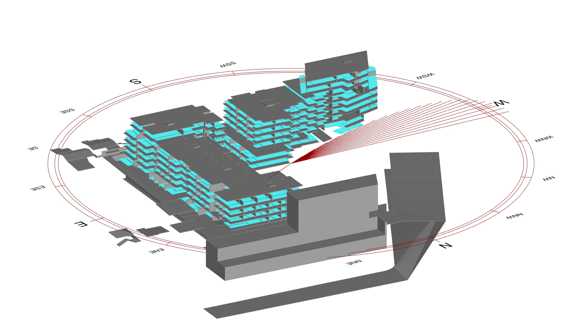
• Set the visualisation input (#37) to ‘Analysis geometry’, and check that all the rooms/masses you want to analyse are shown in Rhino. The colour can be modified by changing the ‘Solar path’ (#38) and ‘Analysis geometry’ colour pickers (#39).

• Set the visualisation input (#37) to ‘Context geometry’, and check that all the context is shown in Rhino. The colour can be modified by changing the ‘Context geometry’ colour picker (#40).

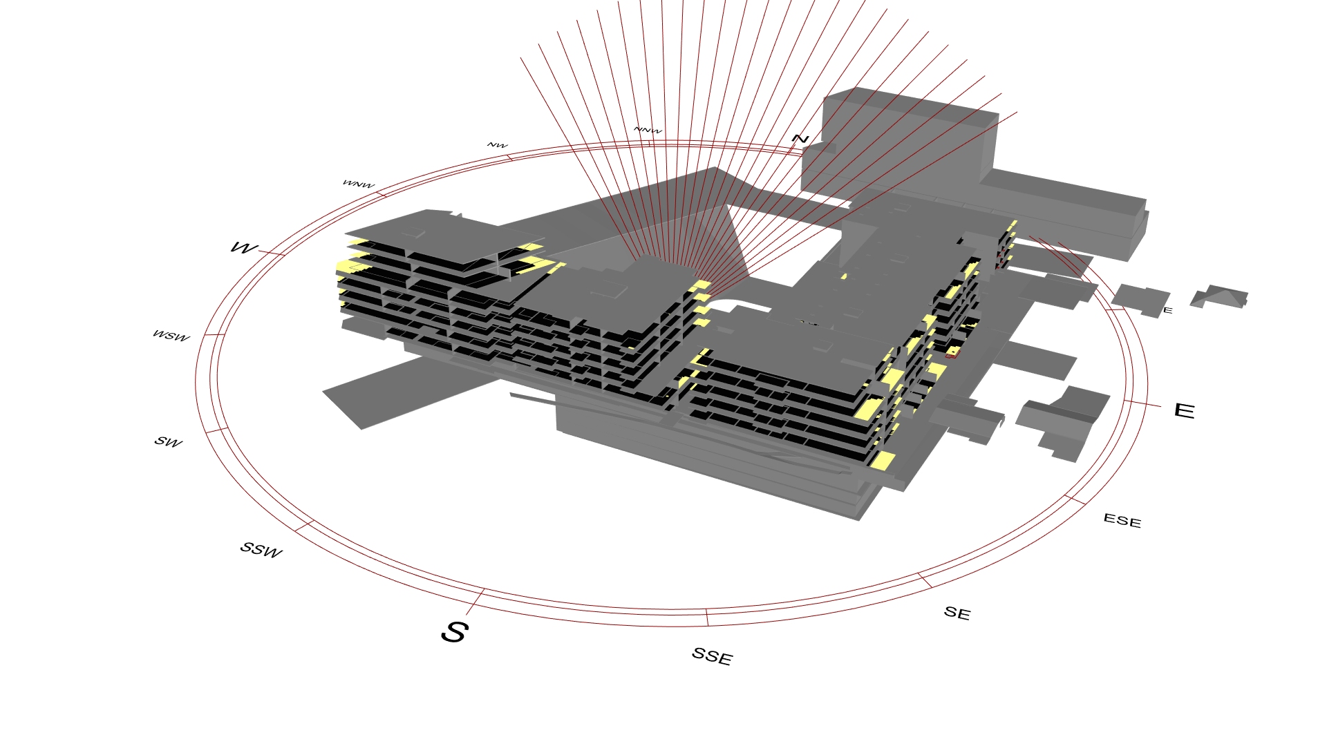
• Set the visualisation input (#37) to ‘Detailed Heatmap’, and check that the analysis is shown correctly in Rhino. The colours can be modified by changing the ‘Detailed Heatmap’ (#41) colour pickers.
• Set the visualisation input (#37) to ‘Simplified Heatmap’, and check that the analysis is shown correctly in Rhino. The colours can be modified by changing the ‘Simplified Heatmap’ (#42) colour pickers.

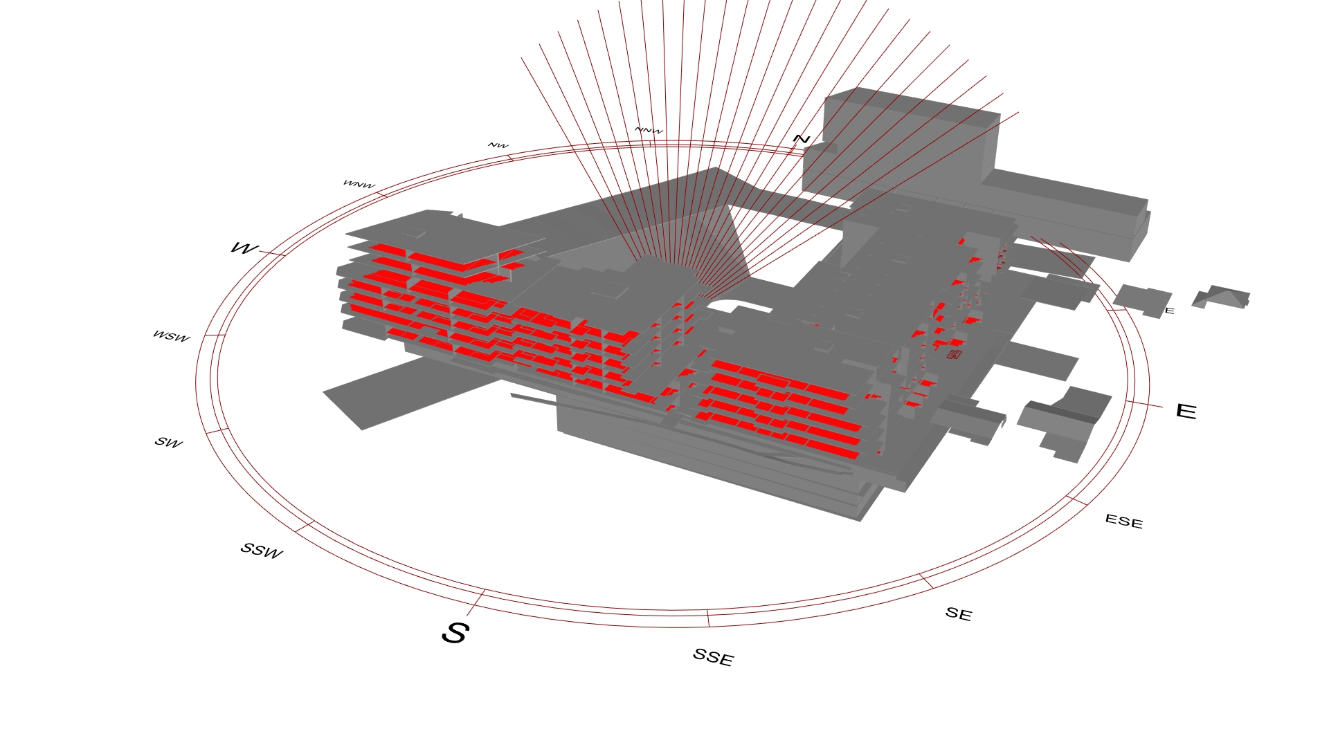
• To see complying vs non-complying , set the visualisation input (#37) to ‘Comply vs non-comply zones’ or ‘Comply vs non-comply room/area’. The colours can be modified by changing the ‘Complying’ (#43) and the ‘Non-complying’ (#44) colour pickers.

• To see the areas that receive no sun, set the visualisation input (#37) to ‘No sun zone’ or ‘No sun room/area’. The colour can be modified by changing the ‘No sun’ colour picker (#45).

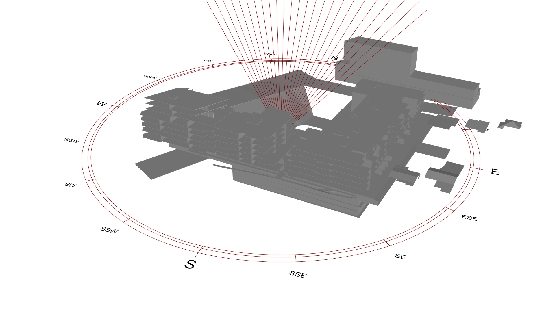
• To see the areas that receive sun at a specific time (#47), set the visualisation input (#37) to ‘Individual sun ray’. The colour can be modified by changing the ‘Individual sun ray’ colour picker (#46). 

Step 14 – Push results to shared parameters

Once the analysis is complete, and you are satisfied with the results, we can push the results into the room’s or area’s shared parameters. Note that this will only work if rooms (analysis type 1) or areas (analysis type 3) were analysed. It will not work if masses (analysis type 2) were analysed.

• Define the yes/no shared parameters to write to for solar compliance and no sun (#48 & #49).
• Enable the ‘Update shared parameters’ toggle (#50).
• The Yes/No parameters for each affected room will be updated. Once this information is in the Revit model, view filters can be set up to visualise each room’s or area’s yes/no compliance. Note that any rooms/areas within a model group will be excluded and shown in the error panel and therefore not updated.

Step 15 – Export results to Excel (optional)

Note that this step will only work if rooms were analysed (analysis type 1). It will not work if masses or areas were analysed (analysis types 2 & 3). The City of Sydney has an Excel template that is often required to illustrate solar access compliance. This is a pre-formatted file setup for 15min intervals. If desired, the script can write the results of the solar access analysis to this file. For this to work, the analysis period much match the Excel file, that is, 9 am – 3 pm at 15min intervals. If certain cells have formulas in them and shouldn’t be overridden by the script, they should be ‘protected’ first.

To export the results:

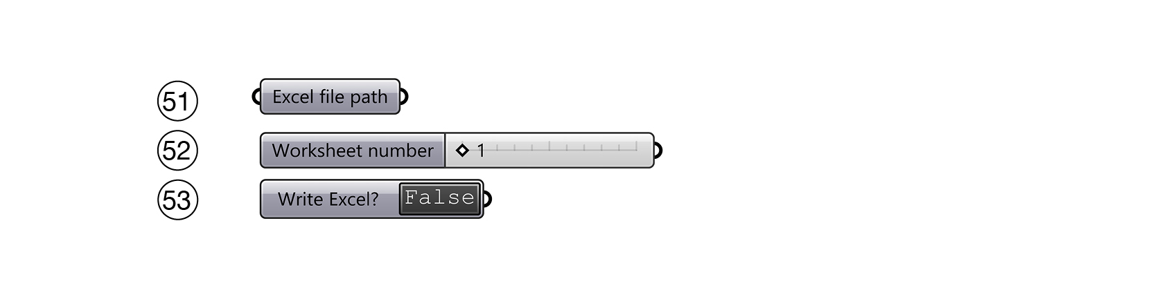
• Right-click on the ‘Excel file path’ component (#51), and select ‘one existing file’. Ensure that the Excel file is blank except for the various header information. 
• Define the worksheet number (#52). The default is set to 1.
• Double-click on the ‘Write Excel’ toggle to enable (#53). This will open the Excel file and populate the data.

As the Excel schedule is structured to require a single value per room per time step, it represents an abstraction of the actual heatmap results. For each room, the script takes the mesh face that receives the most solar access. The centre point of this face is then checked at each time step, and the results are reported. A ‘Y’ (YES) value represents that the mesh face is visible for that particular time step. Note that these values do not mean that the face is visible for the full 15 minutes. Column BB, however, does represent the total sun received.

Because of this method, some parts of the room may be visible during the same time step but not shown on the schedule. Despite this, the data written on the schedule is the most accurate interpretation of the intention of the legislation.

Step 16 – Create Revit elements (optional)

The script provides two creation methods to visualise the solar access heatmap in Revit, both using DirectShapes. DirectShapes are generic Revit elements that can contain and categorise arbitrary non-parametric geometry inside the Revit model.

Common settings

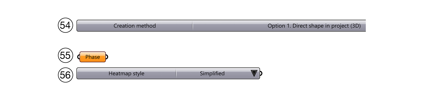
• Define the creation method (#54). Refer below for details of each method.
• Set the phase (#55) for the elements to be created. The heatmap will be created as a DirectShape of category ‘Generic Model’ in Revit.
• Ensure you are on the correct workset. Ideally, this should be a workset that is hidden by default, and only appears where needed.
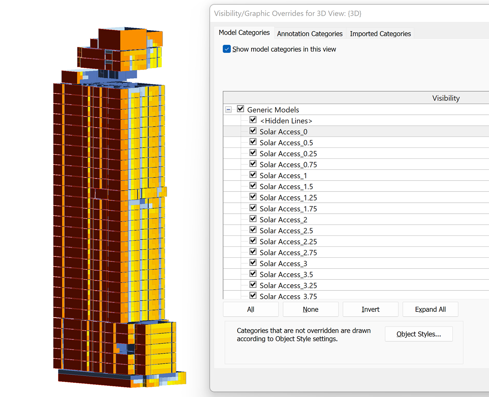
• Also, ensure that the generic model category is visible in Visibility Graphics (VG) otherwise, the results will not be visible.
• Define the heatmap style (#56).

Option 1: DirectShapes in project

• This option is the simplest and fastest creation method where multiple DirectShapes are created in the model, one for each time step result (0hrs, 0.25hrs, 0.5hrs, etc.).
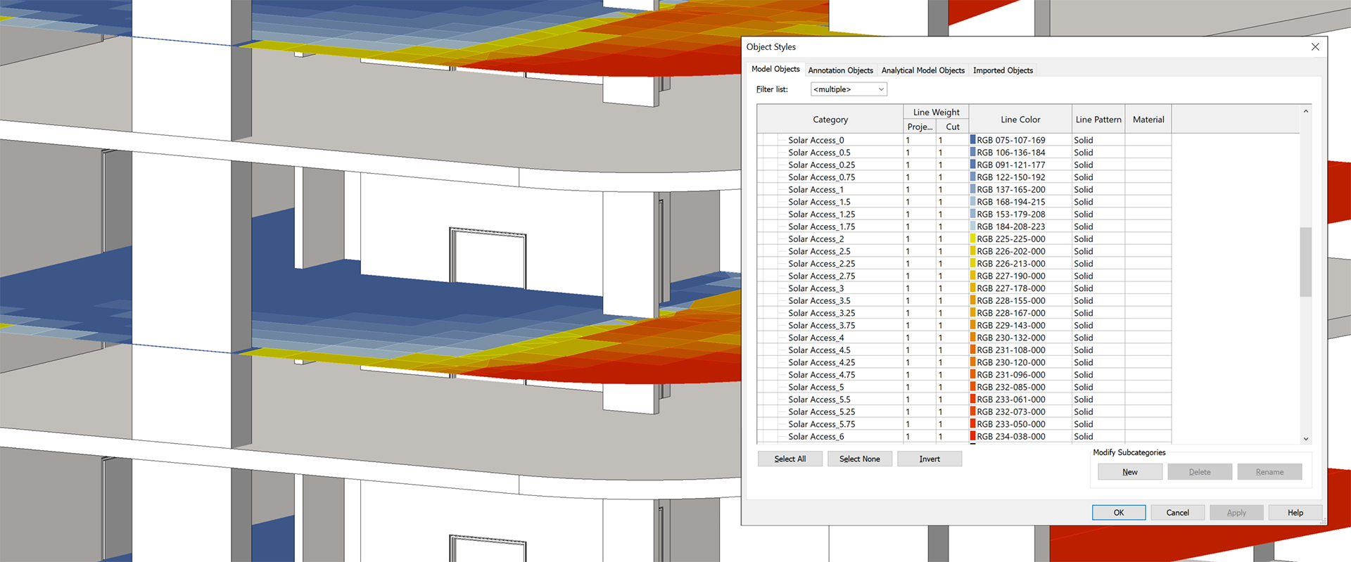
• Corresponding materials are also created and applied to the DirectShape. The material colours will match the script’s colours (#41 or #42).
• To assist in grouping elements, specify a prefixed (#57). Elements will be named ‘Prefix + Result’, for example, ‘Solar Access_2’.
• Note that if you are in Revit 2020, you’ll need to tweak the display mode, otherwise you’ll see the DirectShape edges.

Option 2: Loadable family (preferred)

• Loadable families are best created to provide more control over visibility and file management.
• Loadable families enable the creation of subcategories. As a result, when this option is selected, only a single ‘Generic Model’ family is created, but with multiple subcategories, one for each time step result (0hrs, 0.25hrs, 0.5hrs, etc.). The line colour is also updated so that there are no visible black lines around each DirectShape.
• Corresponding materials are also created and applied to the DirectShape. The material colours will match the script’s colours (#41 or #42).
• Define the generic model template file path (#58). This is typically: C:\ProgramData\Autodesk\RVT 2022\Family Templates\English\Metric Generic Model.rft.
• Define the path to save the family (#59). This location will typically reside in your project folder. Note that the script will automatically load and place the family in the correct location once created.
• Define the level for the loaded family to be placed (#60). Note that this is for (Generic Model) scheduling purposes only, as in any case, the Z-coordinate will be accurate as the ‘Elevation from Level’ parameter will be updated.
• To assist in grouping elements, specify a prefixed (#61). Elements will be named ‘Prefix + Result’, for example, ‘Solar Access_2’.
• Define the family name (#62).

Compute

• Enable the ‘Create Revit elements’ toggle (#63). This operation could take several minutes to complete.

Multiple options

• If you need to run multiple options, all pushed to Revit, care must be taken due to Rhino.Inside.Revit’s built-in element tracking.
• First, ensuring the ‘Create Revit elements’ toggle is still enabled (#63), disable the Grasshopper solver (Solution > Disable solver).
• Next, update the prefix(s) (#57, #61 & #62). The prefix must be different, otherwise, it will override the existing element.
• Finally, you’ll need to disable Element Tracking on the various components creating Revit elements. Use the Jump icon to go to the component area. Right-click on the components (grouped in ‘Tracking’) and set the tracking mode to ‘Disable’.
• Once updated, enable the Grasshopper solver (Solution > Disable solver). Duplicate elements should now be created. When closing the script, you may not wish to save it, depending on how you want the script to run once reopened.

Step 17 – Bake to Rhino (optional)

• To create geometry in Rhino, enable the ‘Bake to Rhino’ toggle (#64).
• Note that re-enabling this multiple times will create duplicates. If this is not desired, delete the layers/geometry in Rhino first before activating.

Step 18 – Reset Boolean toggles

The various compute toggles need to be reset to prevent the script from re-executing automatically once re-opened. However, again care must be taken due to Rhino.Inside.Revit’s built-in element tracking. Otherwise, Rhino elements will be deleted once deactivated.

• First, disable the Grasshopper solver (Solution > Disable solver).
• Next, re-set all of the compute toggles to False (#23, #25, #35, #36, #50, #53 & #63).
• Save the Grasshopper file and close it.

Conclusion

One of the surest ways to design better buildings is to undertake better analyses. However, often analyses are performed outside of the model authoring software, meaning that results tend to get ‘lost’ and fail to create a positive feedback loop. With the release of Rhino.Inside Revit, this need not be an issue. As shown above, numerous environmental analyses, including solar access, can all be performed inside Revit and the results stored within the Revit model.

To find out more about this script or our custom software development service, drop us a line and discover how we can automate your workflows.