AU 2017 exhibition hall: A case study in generative design

In the context of Gartner Hype cycle, it would appear generative design has hit the peak of inflated expectations. If you listen to the hype, there isn’t much generative design can’t do. It is marketed as the process of merely telling the software the results you want, and with your guidance, it arrives at the optimal solution.¹ The truth, however, is that generative design is much more complex, especially if you want meaningful results. This tutorial will explore some of those challenges via a case study – the Autodesk University 2017 exhibition layout by The Living.

What is Generative Design?

Before we begin, it is essential to define what we mean by generative design. The term ‘Generative design’ has been around for some time, and much ink has been spilt debating its definition.² And no doubt some may disagree with this definition. However, first and foremost, generative design is a specific application of computational design. You can think of computational design as the all-encompassing parent category. Generative design is just one application of computational design.

Secondly, generative design is an extension to a parametric model. Where parametric models are generated automatically by internal logic arguments, generative design evaluates the outcome against some criteria (design goal) and then automatically re-runs until the design goal(s) is achieved or optimised. And this brings us to our first important point:

Point #1: There is no magic generative design button

You must codify the underlying logic first before even attempting generative design. This requirement is subject to change given the ever number of companies seeking to make generative design more accessible to the mainstream market.

Solution space

The range of possible outcomes is known as the ‘solution space‘ (or the ‘design space’). If the solution space is too small (high bias), the outcome will be predictable, and the generative design process won’t offer much value. On the other hand, if the design space is too board (high variance), you may be computing unnecessary possibilities – possibly for a very long time! And this takes us to the next important point:

Point #2: Avoid high bias & high variance in the solution space

The real craft is to ensure you have enough control that you get acceptable results, but enough flexibility for some of those results to be unexpected.

Fitness

Results are ranked according to their ‘fitness‘, that is, how well they perform against the design goal(s). Fitness is often inappropriately framed in an overly-simplistic way, such as maximising or minimising area or volume. In reality, however, the real design goal can be hard to articulate, let alone codify. Moreover, they may require many, sometimes conflicting goals. For example, maximising light but minimising heat gain.

If multiple design goals are required, as is often the case, then this is known as Multi-Objective Optimisation (MOO). In the past, we’ve run design studios on this very topic to see how multiple goals could be addressed simultaneously. And this brings us to the final important point:  

Point #3: Defining fitness is hard

Defining fitness

We use intuition and heuristics to assists us in identifying good design. However, this knowledge needs to be made explicit via a set of procedures for a computer to follow. Take the simple task of defining what a good living room should be. A lazy goal might be to say, make it as large as possible. But if you ended up with a ballroom sized living room, would that be good design?

A more nuanced way to define the design goal would be to say, size (area) is important, but the room must be well proportioned (ratio). The room should have enough natural light (lux) and include a window. That window should be of a minimum size and have a view. Adjacency to other rooms is also important. As you can see, the list of requirements could go on and on. But this is what is required if you are to receive meaningful results.

But of course, it doesn’t matter how nuanced a goal is if it asks the wrong question to begin with. A typical application of generative design over the past 12 months has been around social distancing in the workplace.³ Frequently these are presented as a problem of desk proximity. And if you have a small office in a low-rise building, that may be the case. But for others in a high-rise building, it seems a moot point if you have no safe way of accessing the office in the first place. A colleague recently told me that to access their office practising social distancing in the elevators, it would take them until 3pm before everyone was in the office. This example highlights that an optimal solution is only optimal if it asks the right questions to begin with.

Generative Design software

Technically speaking, the term ‘generative design software’ is a bit of a misnomer. I say this because the software isn’t actually generating designs. Sure it might change some input values, but it mainly provides the infrastructure for comparing and evaluating solutions.

Within Grasshopper, there are many possibilities to utilise generative design, including Galapagos, Design Explorer Colibri, Octopus, and Wallacei. Indeed, Galapagos has been around for over a decade now. In Autodesk world, they began with Project Fractal which later turned into Project Refinery. Until last April with the release of Revit 2021, when it became Generative Design for Revit. They all work in more or less a similar way, apart from Galapagos with only calculates a single design goal.

So which software is best for generative design? At Parametric Monkey, we are software agnostic – we use the best tool for the job. To answer the question, I thought it would be useful to create a comparison via a simple case study.

Case study

For the case study, I’ve used the Autodesk University 2017 exhibition layout by The Living. This project was chosen as the case study because it was a real-world project utilising generative design which came to fruition. And secondly, the underlying logic was already documented and publicised. ^{4 5}

The design of the exhibition hall is based on the morphology of urban street layouts. The designers then determined that the most critical goal of the layout was the distribution of foot traffic, such that all exhibitor areas are evenly activated without creating undesirable congestion in any particular location. To capture these desires in the model, they developed two metrics. The first one is called ‘buzz’, and it measures the spatial distribution of high traffic areas in the plan. The second metric is called ‘exposure’, and it measures the average foot traffic around each exhibitor booth. For the purposes of this case study, I have used similar design space parameterisation. However, instead of using buzz and exposure as the fitness, I’ve opted to use the shortest path.

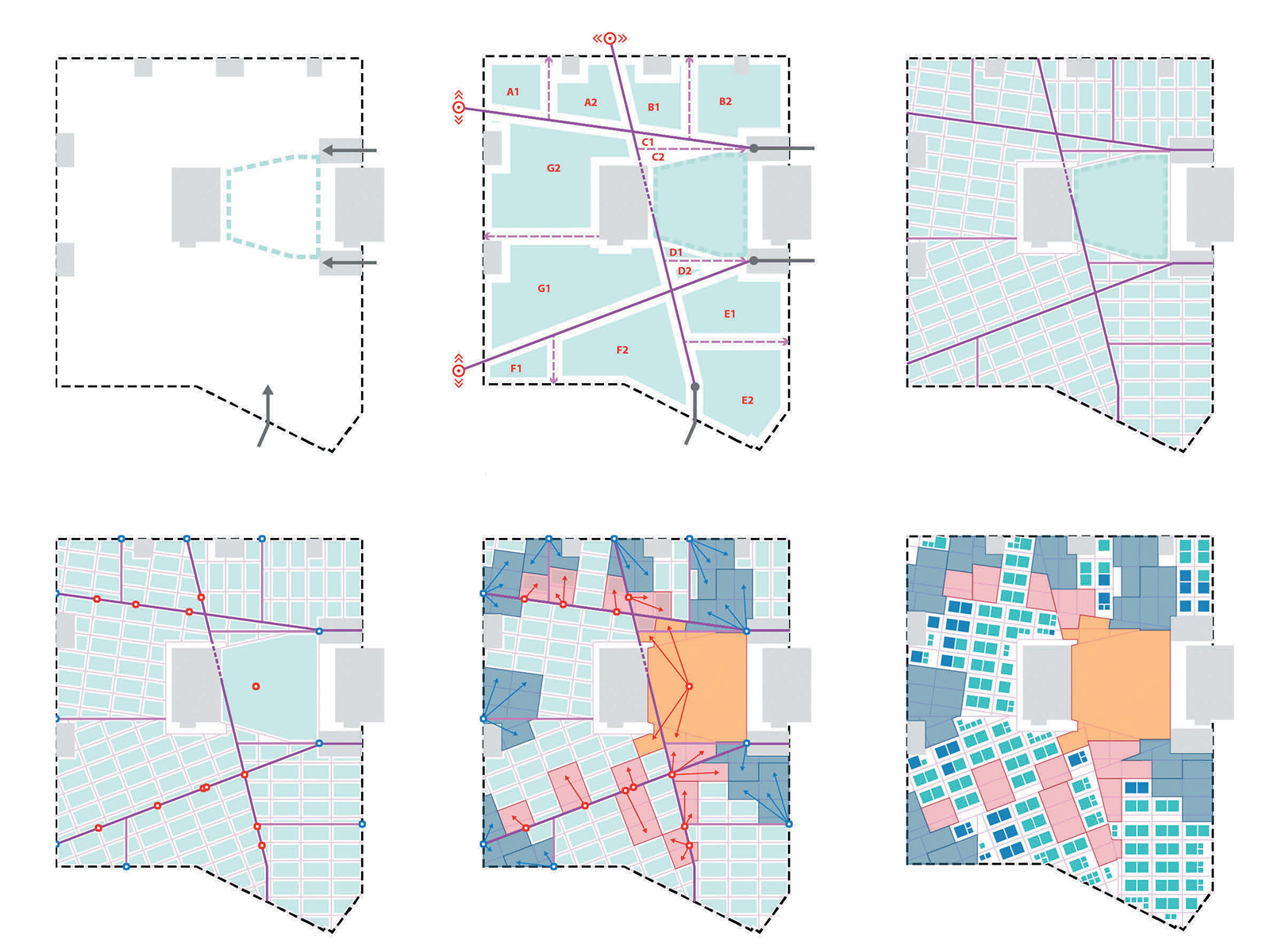
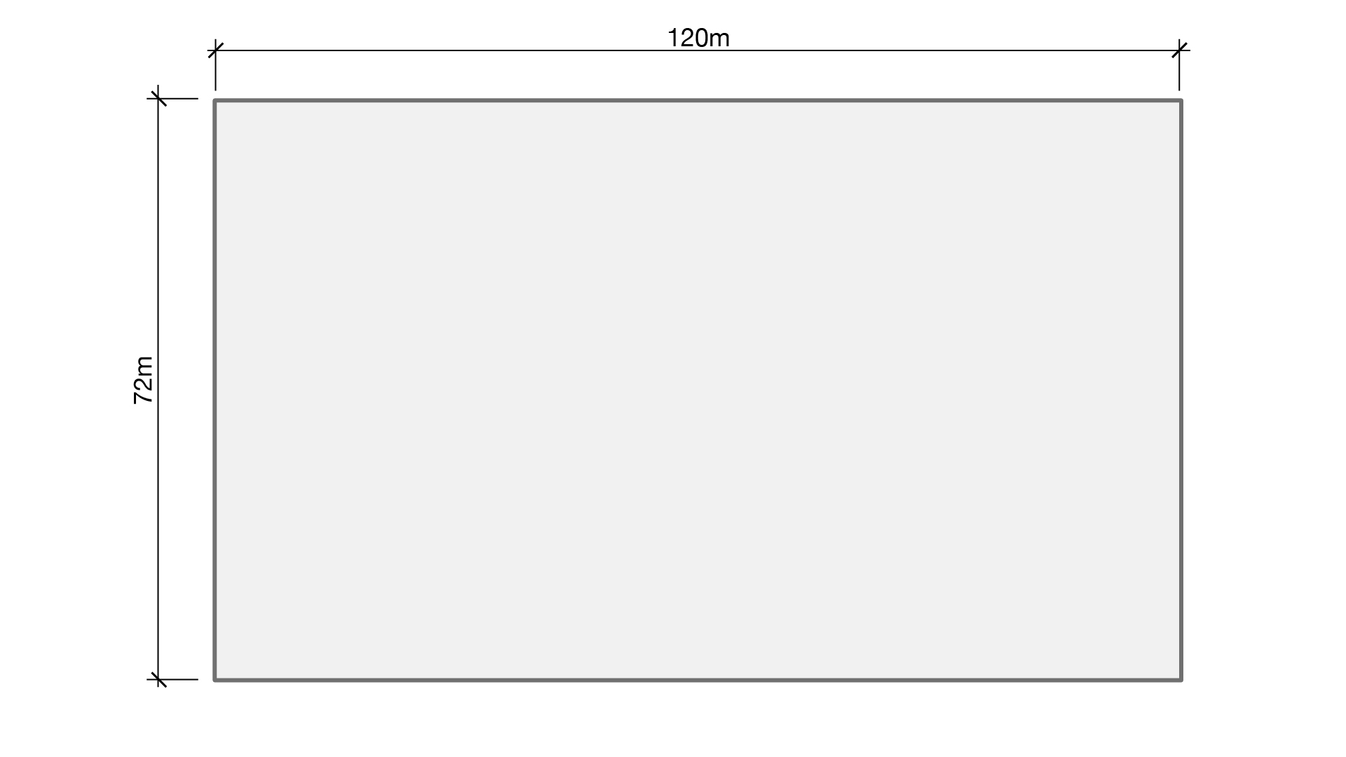
Step 1: Define perimeter boundary

For the case study, I used a simple rectangle 120m x 72m (8,640m²).

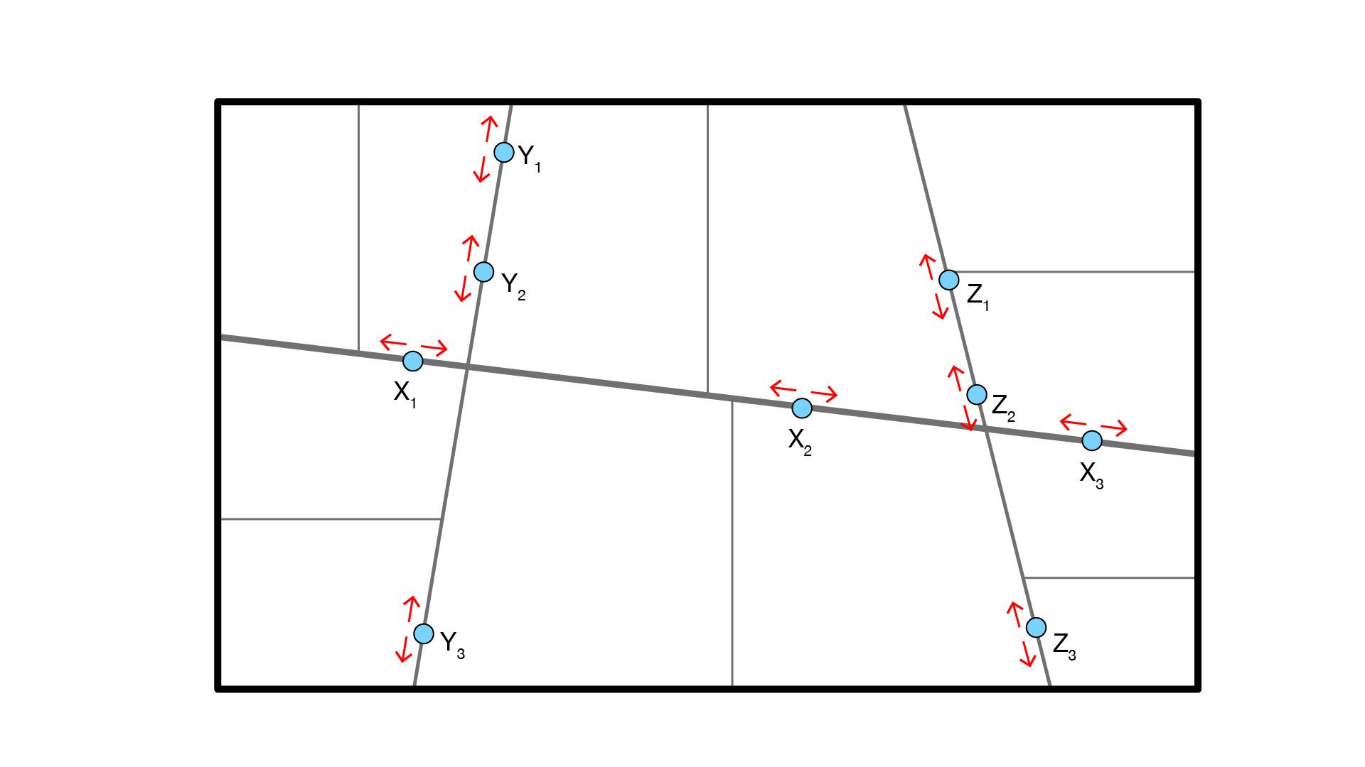
Step 2: Curve parameters

A point on a curve is defined by its t parameter, with the start point t=0, and the end point t=1.

Step 3: Create points by parameters

The major avenue is defined by existing entry and exit points. In comparison, the minor avenues are defined via a line connecting opposite points hosted to the boundary curves.

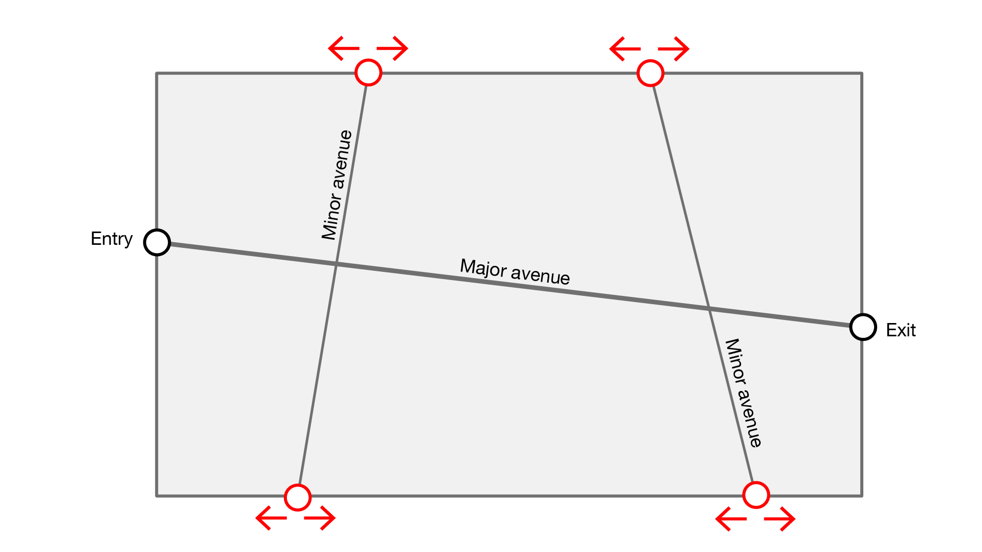
Step 4: Define parameter range

Allowing the start/endpoint to flex across the entire range of t=0 to t=1 may cause undesirable results. For example, the minor avenues may intersect or be too far spaced. The range is therefore reduced from t=0.1 to t=0.45 or t=0.55 to t=0.9 to avoid these outcomes.

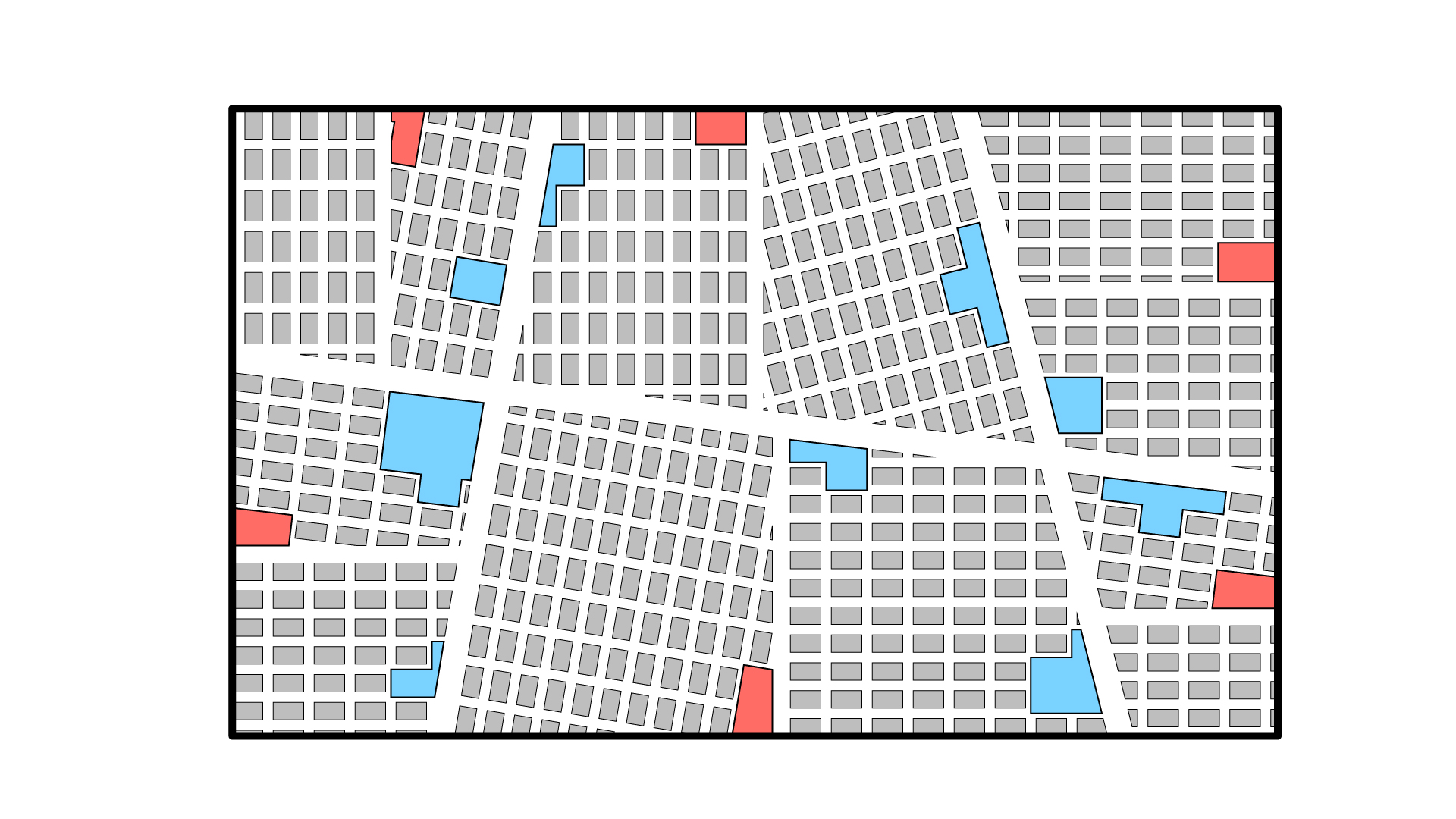
Step 5: Partition floorplan

Using the centrelines of the major and minor avenues, we can offset these lines to create our primary circulation zone. The width of the major and minor avenue is set to 3m. Six zones are therefore created.

Step 6: Subdivisions

Each zone is further subdivided. The midpoint of the perimeter curves are then calculated, and lines are drawn at 90 degrees until they intersect the major/minor avenue.

Step 7: Subdivision partitions

We can offset the subdivision centrelines to create our secondary circulation zone. The width of the secondary circulation is set to 2m. Twelve zones are subsequently created.

Step 8: Calculate setout point

The longest edge of each subdivision is calculated and the start point used for the cells’ setout.

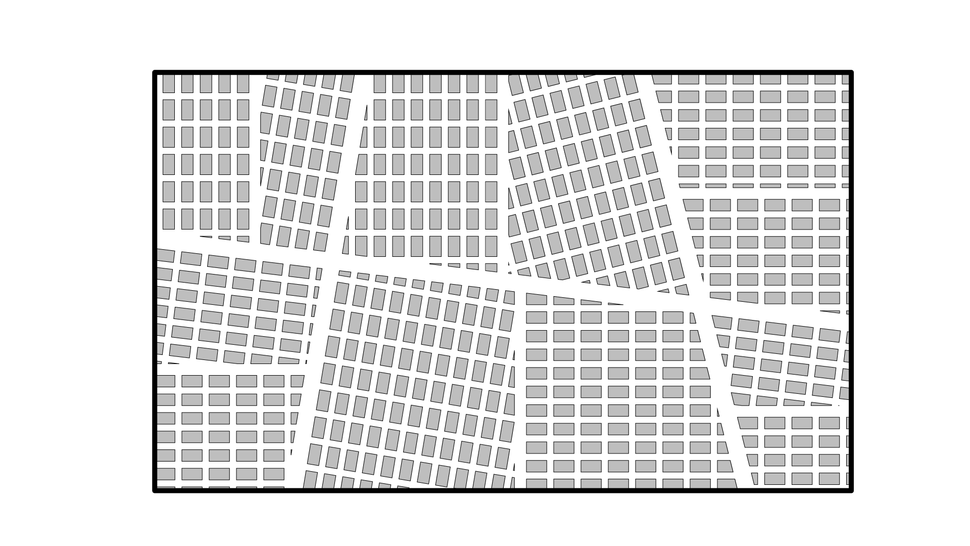
Step 9: Array cells

Cells representing the exhibitor’s booth are arrayed. Each cell has a maximum size of 3.5m x 2m, with 1.2m of spacing between cells. ‘Remainder’ cells which are too small or irregular, can be optionally filtered out.

Step 10: Define food & beverage (F&B) locations

Food and beverage zones are located along the perimeter, at the end of the secondary circulation paths. This decision aims to ensure footfall is distributed and visitors pass by as many exhibitor booths as possible.

Step 11: Define major program locations

Twelve major exhibitor booths are located along the major and minor avenues – three on each avenue. Points are parameterised and can flex from t=0.1 to t=0.9.

Step 12: Create F&B and major program

The nearest cell closest to the F&B (red) and major program (blue) locations is found. The cell is then ‘grown’ by merging adjacent cells until each program’s size requirement is achieved. Program areas range from 19m² to 100m². A constraint is established to ensure cells don’t overlap.

Interlude

At this point in the process, we have a fully parametric model. The avenue and programs’ location can be adjusted, and the area requirements decreased or increased, and the model will flex accordingly. The difference between the Grasshopper script and the Dynamo graph is negligible. But if we were to stop here, this wouldn’t be a generative design model. So let’s continue.

Step 13: Calculate shortest path (define fitness)

Using the entry point, we can calculate the shortest path to each F&B and major program. This route can be achieved in Grasshopper using the Shortest Walk plug-in. This component used the A* search algorithm and requires graph curves, which are the circulation paths, split at each junction. Computing the shortest path is extremely fast, only 30ms.

Dynamo, on the other hand, is much more problematic. Using Autodesk’s Refinery Tool Dynamo package, we can use the ‘PathFinding.ShortestPath’ node. Apart from using the Dijkstra algorithm, the main difference with this node compared to Grasshopper’s ShortestWalk component is that the node requires ‘obstructions’. That is, it is after a list of polygons which represent our cells.

The problem with this is that the node is unnecessarily trying to compute the graph curves itself, even though we already have these calculated elsewhere and could have fed them into the node. The result is that the graph effectively times-out. Given enough time, it might finish computing, but I aborted after several minutes so who knows the final run time. It would seem then, that Dynamo’s dedicated generative design nodes are inadequate for a design this ‘complex’ (ahem).

As a workaround, however, we can use Lunchbox’s ‘Curves.ShortestWalk’ node. This node uses the same algorithm and code as the Grasshopper’s ShortestWalk component. Although, interestingly it takes around 22 times longer to compute at 683ms.

Once calculated, the shortest path’s value can be fed into our generative design analysis to either maximise or minimise. For some, getting to food as quickly as possible during a break should be the priority. For an exhibitor’s perspective, adopting the Ikea model to maximise exposure is more desirable. Hence the option to minimise or maximise. For this case study, I opted to minimise the distance.

Step 14: Graph adjustments (Dynamo only)

If you are using Generative Design for Revit, you’ll need to make some adjustments to your Dynamo graph. These adjustments ensure no transactions are made until a preferred design is chosen. Transactions modify the Revit project whereas what we want to do, is create ‘abstract’ geometry (points, lines, curves, etc.), choose an option, and then generate Revit elements (floors, walls, filled regions etc.). To do this, we need to use the ‘Data.Remember‘ and the ‘Data.Gate‘ nodes.

Data.Remember is used to store information from Revit. From a technical perspective, the Revit geometry is cached meaning that future iterations can be run without Revit. In our case, I’m using model lines to define the perimeter boundary, so these need to be feed into Data.Remember.

The Data.Gate node controls the flow of data back into Revit. By default, it must be set to ‘Close’, meaning no data will flow through during the iteration process. Only once a design is accepted will it toggle to ‘Open’, allowing data to follow and enabling the creation of Revit elements. In our case, I’m using filled regions to represent the cells (exhibitor booths), and model lines to represent the shortest path.

Additionally, like in Dynamo Player, we need to ensure that all inputs are renamed and right-clicked to enable the ‘Is Input’ option. The same also needs to be done for any output nodes (except obviously you need to set the ‘Is Output’).

Step 15: Creating a study (Dynamo only)

The final step is to create a study. Depending on the solver method chosen, you may receive one or many studies. Interesting, while the UI remembers the settings from Data.Remember (that is, our model line inputs), it doesn’t seem to remember the settings for Data.Gate (that is, our filled region outputs). The other point to remember is that the analysis is being run on your desktop and Revit needs to remain open. No doubt in the future, this will change to a cloud-based token system as per other Autodesk analysis tools.

Once completed, chose the study you wish to accept and press the Create Revit Elements button. This action will enable the Data.Gate node and create the Revit elements.

Compute comparison

There is much to like about Generative Design for Revit. The UI is clean and user friendly, and it integrates seamlessly into Revit. But this is also its downfall. Let me explain. Generative Design for Revit is structured to run independently from Revit (using the ‘Data.Remember’ and ‘Data.Gate’ nodes). But it is still using Dynamo to compute the main body of the graph. Despite all the performance improvements the Dynamo team have made recently, it is still far slower than Grasshopper. Here is a comparison of the total compute time:

Grasshopper: 4.8 sec
Dynamo: 25 sec

As you can see, Dynamo (v2.6) is 5 times slower than Grasshopper (v1.0). If you plan on just running a couple of iterations, this discrepancy is probably no big deal. On the other hand, if you plan on running hundreds or thousands of options, then there will be a massive time difference between the two. I’ll be the first to concede that both versions could be better optimised to run faster. But this doesn’t take away from the fact that using the same or very similar operations takes dramatically different run times between the two software.

In my opinion, if we are already decoupling the main ‘grunt work’ from the Revit element creation, it makes more sense to use the fastest and most efficient software. As such, depending on your design, it is likely going to be much quicker running a Grasshopper script and then pushing the results into Revit using Rhino.Inside Revit. Of course, if you’re not proficient with Grasshopper than this method won’t be more efficient. But if you do decide to go down the Dynamo route, keep in mind it will take longer to compute.

Generative design animation

The second major flaw I see with Generative Design for Revit is that you don’t see the design changing through the iteration process. And let’s be honest, for many, that is generative design. We were sold animations like this one, but what we got were static outputs.

Of course, it’s obvious there has been a lot of post-processing that has gone into the video above. But at least in Grasshopper, you receive some visual feedback. On the other hand, Dynamo for Revit is very much a black box, spitting out results once complete. This technical limitation is not insurmountable, and hopefully, we’ll see Autodesk develop more functionality around comparing options, including in-built spider graphs.

Conclusion

Generative design as a methodology is exceptionally compelling. It has the power to unearth both improved and novel solutions compared to current design methodologies. But as Peter Parker famously said, “with great power comes great responsibility.” There is no magic generative design button and defaulting to pre-made, overly reductive design goals, will only diminish the design outcome, not improve it. If we want meaningful results, we must take the process of defining fitness and the solution space seriously. 

Contrary to popular thought, generative design doesn’t remove the designer from the design process. If anything, generative design forces the designer to be much more intentional, by demanding that their design goals be explicit. As we’ve seen, defining fitness is hard – but not impossible. We’ll talk some more about ‘knowledge elicitation‘ – the process of capturing unstructured and informal knowledge based on experience – in a follow-up post. But suffice to say, having an expert guide you through the process of ensuring you ask the right questions and codifying your design goals, is a smart move if you want to get the most out of generative design. So think about what your design goals really are, and start generating!

References

¹ Autodesk. (2018). Demystifying generative design.

² Stasiuk, D. (13 June 2018). Design modeling terminology.

³ Autodesk. (22 Jul  2020). Socially distant spaces: New approaches with generative design.

⁴ Nagy, D. et al (2017). Beyond heuristics: A novel design space model for generative space planning in architecture. ACADIA: Disciplines & Disruption.Proceedings of the 37th Annual Conference of the Association for Computer Aided Design in Architecture (ACADIA), Cambridge, 2-4 Nov 2017, pp. 436- 445.

⁵ Villaggi, L. & Nagy, D. (2017). Generative design for architectural space planning: The case of the Autodesk University 2017 layout. Proceedings of the Autodesk University, Las Vegas, 14-16 Nov 2017.

⁶ Nagy, D. et al (2017). Beyond heuristics: A novel design space model for generative space planning in architecture. ACADIA: Disciplines & Disruption.Proceedings of the 37th Annual Conference of the Association for Computer Aided Design in Architecture (ACADIA), Cambridge, 2-4 Nov 2017, pp. 436- 445.

⁷ Autodesk (2019). Generative design primer.

References

1 Autodesk. (2018). Demystifying generative design.
2 Stasiuk, D. (13 June 2018). Design modeling terminology.
3 Autodesk. (22 Jul 2020). Socially distant spaces: New approaches with generative design.
4 Nagy, D. et al (2017). Beyond heuristics: A novel design space model for generative space planning in architecture. ACADIA: Disciplines & Disruption.Proceedings of the 37th Annual Conference of the Association for Computer Aided Design in Architecture (ACADIA), Cambridge, 2-4 Nov 2017, pp. 436- 445.
5 Villaggi, L. & Nagy, D. (2017). Generative design for architectural space planning: The case of the Autodesk University 2017 layout. Proceedings of the Autodesk University, Las Vegas, 14-16 Nov 2017.
6 Nagy, D. et al (2017). Beyond heuristics: A novel design space model for generative space planning in architecture. ACADIA: Disciplines & Disruption.Proceedings of the 37th Annual Conference of the Association for Computer Aided Design in Architecture (ACADIA), Cambridge, 2-4 Nov 2017, pp. 436- 445.
7 Autodesk (2019). Generative design primer.
4 Comments
Fabio Loretti Oliveira
Good article, mate. Thanks for posting it.
Paul Wintour
Thanks mate. Glad you found it useful.
Mikel Martinez
Thank you very much, for those of us who are trying to go deeper into this field, clear articles like this one are very motivating. I’m going to use it as a base to try a couple of things!
You’re welcome. I’m glad you found it useful.